VAE: Variational Autoencoder

An autoencoder is a type of neural network used to learn efficient representations of data, typically for the purpose of dimensionality reduction or feature learning.

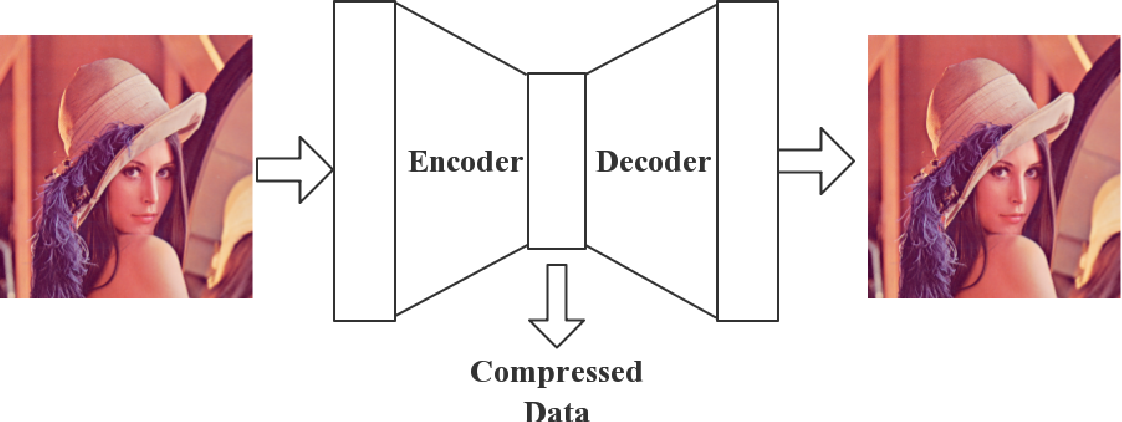
At its core, an autoencoder has two main parts:

• Encoder: The encoder takes the input data and compresses it into a smaller, more compact representation, often called the "latent space."

• Decoder: The decoder then takes this compressed representation and tries to reconstruct the original input data from it.

Training an Autoencoder

The training process involves minimizing the difference between the original input and the reconstructed output, which encourages the autoencoder to learn meaningful features of the data in the latent space. Say for an image, the pixel-wise difference between the input and reconstructed images is used to calculate the Reconstruction loss and update the weights of the network.

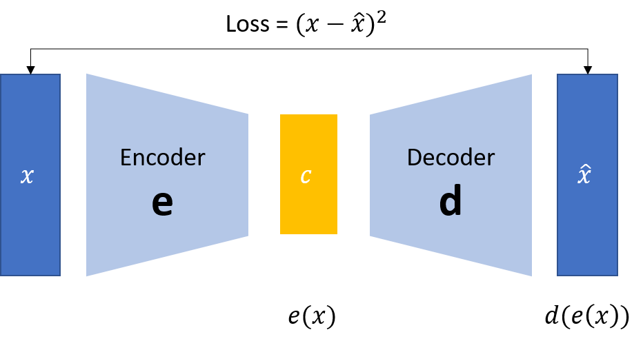
Reconstruction loss is typically calculated using metrics such as mean squared error or binary cross-entropy.

By doing this, autoencoders can learn to ignore noise and focus on the most important aspects of the data.

Introducing Variational Autoencoder (VAE)

A variational autoencoder (VAE) is a more advanced type of autoencoder that adds an extra layer of complexity to this process. Instead of just learning a fixed representation in the latent space, a VAE learns the parameters of a probability distribution representing the data. This means that instead of encoding an input as a single point, it is encoded as a distribution over the latent space.

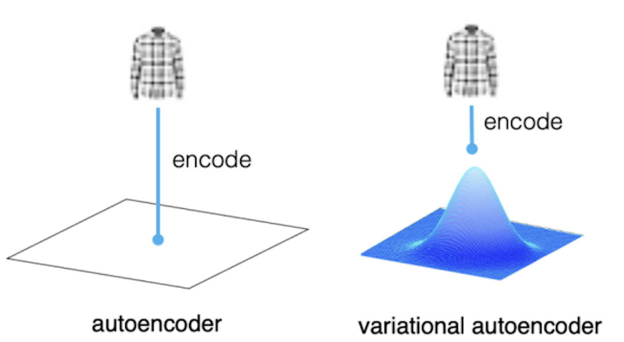
Autoencoder encodes input as a single point in the latent space. VAE encodes input as a distribution over the latent space.

This probabilistic approach allows VAEs to generate new data that is similar to the original input data, making them useful for tasks like image generation and anomaly detection. By learning the underlying distribution of the data, VAEs can produce a diverse range of outputs, providing a more flexible and powerful tool for understanding and manipulating complex data.

VAE Architecture

With that basic idea of a VAE in mind, let's take a closer look at the architecture and training process of a variational autoencoder.

Encoder: Learning a Distribution

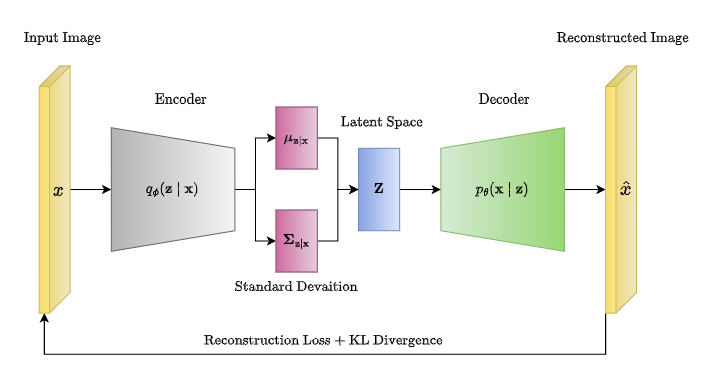
In a VAE unlike autoencoder, the encoder doesn't directly produce a single compressed representation of the input data. Instead, it outputs the parameters of a probability distribution, typically a Gaussian distribution. This means the encoder gives us two things for each input:

Mean (μ): The center of the distribution.

Variance (σ²): The spread or uncertainty of the distribution. These parameters describe a range of possible values in the latent space that the input could correspond to, instead of just a single point.

Sampling: Adding Randomness

Now, we have a distribution for each input, but we need a specific point in the latent space to send to the decoder. This is where sampling comes in. We randomly pick a point from the distribution given by the encoder. This process adds randomness to the model, which is important for generating diverse outputs. But, there's a problem with this direct sampling approach.

Backpropagation Issue in Direct Sampling

• The encoder outputs parameters (mean μ and variance σ²) of a distribution, and then normally during a forward pass, a latent variable z is sampled directly from this distribution.
• Gradients do not flow through a random node (check figure above). The direct sampling is problematic because it introduces randomness into the computational graph, making it difficult to compute gradients during backpropagation. Since, it is a stochastic (random) process. This means that the exact value of z is not a deterministic function of the encoder's parameters. It's like rolling a dice; you can't predict the exact outcome based on the properties of the dice.
• Because of this randomness, we can't directly compute the gradient of the loss function with respect to the encoder's parameters. It's like trying to find out how changing the weight of the dice would affect the outcome of a roll; there's no direct relationship.

Therefore, to address this issue in sampling, we typically use a technique called the Reparameterization Trick. Now, let's see how that works.

Reparameterization Trick

Instead of sampling z directly, we first sample a random variable ϵ from a standard normal distribution (mean 0 and variance 1).

We then use ϵ to compute z as: z=μ+σ×ϵ

This way, the randomness is "reparameterized" and separated from the network's parameters. The sampling process is now differentiable with respect to μ and σ, allowing gradients to flow back through the network during backpropagation.

Decoder: Reconstruction

The decoder takes the sampled point from the latent space and tries to reconstruct the original input data. The goal is to make the reconstructed output as close as possible to the original input.

Training: Balancing Act

During training, we want our VAE to do two things:

• Reconstruction: We want the reconstructed outputs to be close to the original inputs. This ensures that our latent space representations are meaningful.

• Regularization: We want the distributions learned by the encoder to be similar to a standard normal distribution. This prevents the model from just memorizing the inputs and encourages it to learn useful and generalizable features.

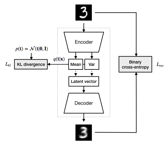
Loss Function

We achieve the balance between the above two objectives by constructing a loss function that combines a Reconstruction Loss L_rec (like mean squared error) and a Regularization Loss L_KL called the Kullback-Leibler (KL) divergence, which measures the difference between the learned distribution and a standard normal distribution.

In summary, a VAE learns to represent data as distributions in a latent space, samples from these distributions to add randomness, and then reconstructs the input from these samples, all while balancing reconstruction quality with distribution regularity.