CLIP: Bridging Vision and Language in AI
Table of Contents
- Introduction
- CLIP Architecture
- Text-encoder Architecture
- Image-encoder Architecture
- Similarity Score
- Training
- Contrastive Learning
- Loss Function
Introduction
Today, Image generation models such as Stable Diffusion and Midjourney are surprising the world with their ability to generate high-quality images based on textual prompts. Many people wonder how these models are able to understand a piece of text and visualise it. And, this is exactly what we will uncover in this article.
We are, from a very young age, able to understand and make sense of the world around ourselves by using our senses, primarily through vision. We observe objects, people, and events and gradually learn to map these visual experiences to words and language.
For example, when a child sees a red round fruit, they eventually learn to associate it with the word 'apple'. This process involves not just the recognition of shapes and colors but also the understanding of context and the relationships between different objects.
As children grow, their ability to map what they see into language becomes more sophisticated. They learn to describe not just objects but also actions, emotions, and abstract concepts. This development is crucial for communication and learning, as it allows children to share their experiences and thoughts with others and to build on their existing knowledge.
CV and NLP: Two Separate Domains
Traditionally, computer vision and natural language processing (NLP) have been treated as separate domains, with different models and techniques used. However, CLIP (Contrastive Language-Image Pretraining) takes a different approach by jointly learning from images and their associated text descriptions.

CLIP is a model that can understand and connect the content of images with corresponding words and sentences. For instance, when presented an image of a dog, CLIP can associate it with textual descriptions like "a brown dog" or "a pet playing in the park."
This ability to link visual and textual information makes it useful for various applications, from image search and classification to more complex tasks like visual question answering and most importantly image generation based on textual prompts (Stable Diffusion, DALL-E, Midjourney).
So, how does CLIP do this mapping?
CLIP is trained using an approach where it is trained to associate images and their textual descriptions and negative samples. This is called contrastive learning, where the model learns to pull together similar pairs and push apart dissimilar pairs or in other words, learns the contrast between positive and negative samples.
1. General Architecture of CLIP
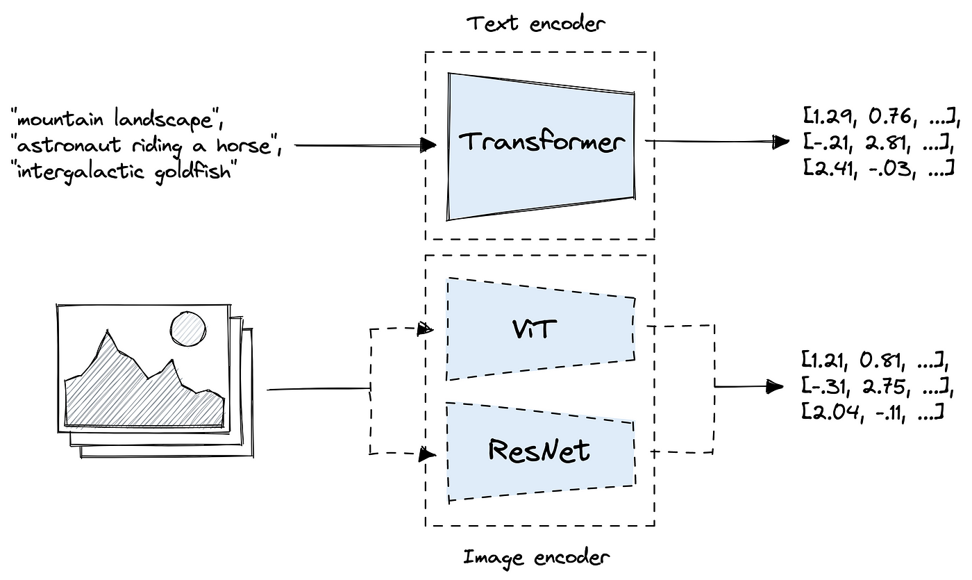
CLIP is a model that learns to associate images and text by converting them into a common representation space and then measuring the similarity between them. This is done using separate encoders for text and images, which convert them into fixed-size embeddings that can be compared using a simple dot product. So, let's look at how CLIP does this.
- Text Encoder: Tokenizes the text and converts it into a fixed-size embedding of 512 dimensions.
- Image Encoder: Converts the image into a fixed-size embedding of the same size (512 dimensions).
- Measuring Similarity: Once the text and image are converted into a common representation space, CLIP uses a simple dot product to measure the similarity between the two.
So, to summarize, CLIP learns to associate images and text by converting them into a common representation space and then measuring the similarity between them.
import torch
import clip

model, preprocess = clip.load(name="ViT-B/16", device=device)
To achieve this, both images and text would be converted into a common representation space, where the similarity between them can be measured. This is done using different encoders for image & text, trained to produce same-size embeddings.
1.1. Text Encoder Architecture
Text is tokenized first and then a text encoder converts it into a fixed-size embeddings. Since the advent of transformers, models such as BERT, GPT-3, and T5 have been used to encode text into semantic embeddings.
import clip

# Load the model and tokenize the text
model, _ = clip.load(name="ViT-B/16")
text = clip.tokenize(["a diagram", "a dog", "a cat", "a place"]).to(device)

with torch.no_grad():
    text_embeddings = model.encode_text(text)

print(text_embeddings.shape)
# Output: torch.Size([4, 512])
Once the text is tokenized using CLIP's tokenizer using clip.tokenize method, the model.encode_text method is used to convert the input texts into a fixed-size 512-dimensional embedding. This embedding can then be used to measure the similarity between different texts.
Once the training is completed, only the text encoder is used in Stable Diffusion and Dall-E to convert the text prompts into embeddings for conditioning the image generation process
The text encoder is a Transformer (Vaswani et al., 2017) [4] with the architecture modifications described in Radford et al. (2019). As a base size, a 63M-parameter 12-layer 512-wide model is used with 8 attention heads. The transformer operates on a lower-cased byte pair encoding (BPE) representation of the text with a 49,152 vocab size (Sennrich et al., 2015) [5].
For computational efficiency, the max sequence length was capped at 76. The text sequence is bracketed with [SOS] and [EOS] tokens and the activations of the highest layer of the transformer at the [EOS] token are treated as the feature representation of the text which is layer normalized and then linearly projected into the multi-modal embedding space. Masked self-attention was used in the text encoder to preserve the ability to initialize with a pre-trained language model or add language modeling as an auxiliary objective, though exploration of this is left as future work.
Note that the Transformer architecture used here would be encoder-only (such as that used in BERT) as text embeddings need to be generated from the input text prompts. This is different from the decoder-only architecture used in auto-regressive LLMs such GPT-3 which generate the next token in the sequence.
Now, for comparing these embeddings with images, we need to convert images into a similar 512-dimensional embedding space. So, this is where the Image Encoder comes into play.
1.2. Image Encoder Architecture
Image encoder is trained to convert raw images into a fixed-size vector representation. Models like ResNet, Vision Transformer (ViT), and EfficientNet have been used to encode images into a fixed-size vector representation.
import clip
import torch

# Load the model and preprocessing function
model, preprocess = clip.load(name="ViT-B/16")
image = preprocess(Image.open("dog.png")).unsqueeze(0).to(device)

with torch.no_grad():
    image_embeddings = model.encode_image(image)

print(image_features.shape)
# Output: torch.Size([1, 512])
Now, the model.encode_image method is converts input image into a similar 512-dimensional embedding space. With both text and image embeddings in the same space, CLIP can measure the similarity between them.
So, there were 9 different variants of CLIP trained by OpenAI each with a different image encoder architecture. The ones where the image encoder was Resnet-based ones were named with RN prefix and Vision Transformer-based ones were named with ViT prefix.
- RN50
- RN101
- RN50x4
- RN50x16
- RN50x64
We train a series of 5 ResNets and 3 Vision Transformers. For the ResNets we train a ResNet-50, a ResNet-101, and then 3 more which follow EfficientNet-style model scaling and use approximately 4x, 16x, and 64x the compute of a ResNet-50. They are denoted as RN50x4, RN50x16, and RN50x64 respectively.
- ViT-B/32
- ViT-B/16
- ViT-L/14
- ViT-L/14@336px
For the Vision Transformers we train a ViT-B/32, a ViT-B/16, and a ViT-L/14. For the ViT-L/14 we also pre-train at a higher 336 pixel resolution for one additional epoch to boost performance similar to FixRes (Touvron et al., 2019). We denote this model as ViT-L/14@336px.
-- Excerpt from the OpenAI's CLIP paper
1.3. Similarity Score
Once the text and image are converted into a multi-modal embedding space (512-dimensional), a simple dot product is used to measure the similarity between the two.
# Calculate dot-product between text & image vector embeddings
# Then apply softmax to get probs
logits_per_image = F.softmax(torch.matmul(image_embeddings, text_embeddings.t()), dim=1)
logits_per_image
2. Training
CLIP is trained using a contrastive learning approach, where it learns to associate images and text by pulling together similar pairs and pushing apart dissimilar pairs. This is done using a large dataset of images and their associated text descriptions.
2.1. Contrastive Learning
Contrastive learning is a technique used to learn a representation space where similar samples are pulled together and dissimilar samples are pushed apart. This is done by comparing positive pairs (similar samples) and negative pairs (dissimilar samples) and optimizing the model to minimize the distance between positive pairs and maximize the distance between negative pairs.
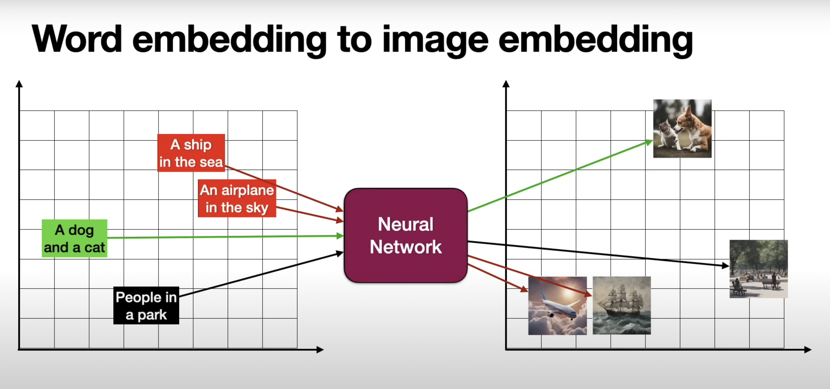
Text and image embeddings are compared using a dot product, and the model is trained to maximize the similarity between positive pairs (images and their associated text) and minimize the similarity between negative pairs (images and random text).
2.2. Loss Function
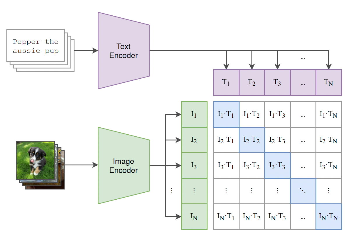
Given a batch of N (image, text) pairs, CLIP is trained to predict which of the NxN possible (image, text) pairings across a batch actually occurred. To do this, CLIP learns a multi-modal embedding space by jointly training an image encoder and text encoder to maximize the cosine similarity of the image and text embeddings of the N real pairs in the batch while minimizing the cosine similarity of the embeddings of the N2 - N incorrect pairings.
The cross-entropy loss function now has to maximize the similarity between correct pairs and minimize the similarity between incorrect pairs.
Correct pairings = N pairs (Maximize similarity)
Incorrect pairings = N2 - N pairs (Minimize similarity)
# Calculate the loss on a batch of N (image, text)
# pairs using cross-entropy loss
import numpy as np

# scaled pairwise cosine similarities [n, n]
logits = np.dot(Image_embeddings, Text_embeddings.T) * np.exp(t)

# Symmetric loss function for text and image
labels = np.arange(n)
loss_i = cross_entropy_loss(logits, labels, axis=0)
loss_t = cross_entropy_loss(logits, labels, axis=1)
loss = (loss_i + loss_t)/2
This batch construction technique and objective was recently adapted for contrastive (text, image) representation learning in the domain of medical imaging by Zhang et al. (2020) [3].
References
- Alec Radford, Jong Wook Kim, Chris Hallacy, Aditya Ramesh, Gabriel Goh, Sandhini Agarwal, Girish Sastry, Amanda Askell, Pamela Mishkin, Jack Clark, Gretchen Krueger, Ilya Sutskever. Learning Transferable Visual Models From Natural Language Supervision. arXiv:2103.00020
- Hugo Touvron, Andrea Vedaldi, Matthijs Douze, Hervé Jégou. FixRes: Fixing the train-test resolution discrepancy. arXiv:1906.06423
- Yuhao Zhang, Hang Jiang, Yasuhide Miura, Christopher D. Manning, Curtis P. Langlotz. Contrastive Learning of Medical Visual Representations from Paired Images and Text. arXiv:2010.00747
- Ashish Vaswani, Noam Shazeer, Niki Parmar, Jakob Uszkoreit, Llion Jones, Aidan N. Gomez, Lukasz Kaiser, Illia Polosukhin. Attention is All You Need. arXiv:1706.03762
- Rico Sennrich, Barry Haddow, Alexandra Birch. Neural Machine Translation of Rare Words with Subword Units. arXiv:1508.07909